V.N.Maximov, N.G.Bulgakov and A.P.Levich

Proposing methods require two groups of techniques to be developed. The first one includes integrated methods for estimating ecosystem conditions using the norm-pathology scale. The second group contains methods of searching for and pattern recognition of the boundaries between the fields of normal and pathological ecosystem functioning in multidimensional space of environmental factors. These boundaries have been named the ecologically tolerable levels (ETL) of disturbing influences. Proposing method allows to calculate ETL values not only for chemical substances, but also for heat pollution and consequences of climate changes, for environment acidification and alkalinization, for water expenditure rates and other influences. The method is useful for prediction and extrapolation of ecosystem conditions according to anthropogenic influencing scenarios.

1. Concept of ecological tolerance and biotic

approach to realization of environmental control

The assessment of ecological state of natural objects (ecological diagnostics), introduction of admissible levels of anthropogenic influences (ecological standardisation) and detection of consequences of the various biota disturbing scenarios (ecological prediction) are the main tasks of the system of ecological control. In the whole territory of former USSR this system is based on the concept of maximum admissible concentrations (MAC) of pollutants. The MAC values are used in solution of all tasks of an ecological control mentioned above. Particularly, the exceeding of MAC forms the basis for unsuccessful assessment of ecosystem state. The MAC standards are determined in laboratory conditions during short-term (days) and chronic (weeks) experiments with isolated populations of organisms, belonging to small number of selected test species, and using limited set of physiological and behavioural responses. The evaluation of natural objects state by MAC levels is an actually unjustified extrapolation of test organisms tolerance borders in relation to isolated influences on multispecific ecosystems, where complicated complexes of tens and hundreds factors of most different nature are operating, on ecosystems being (unlike standard laboratory populations) in completely various background conditions of functioning [3].

The concept of an ecological tolerance proposing admissible levels of influences for biotic part of real ecosystems could be alternative to the methodology of MAC, which is biologically based on existence of tolerance limits for separate organisms. According to the offered concept [22], for any ecological system it is possible to find such limits of the ecological factors variation, at which indications, distinguishing this ecosystem from another, adjacent ecosystems, save their relative stability. In indicated sense it is possible to identify limits of ecological tolerance with borders, inside which the ecosystem state is considered as normal. Then in relation to xenobiotic pollutants the lower limit of tolerance is established automatically: this is their complete absence in ecosystem. The upper limit of tolerance may be considered as ecologically tolerable level of pollution.

The idea about tolerance limits is well-known in ecology, but only in the application to individual organisms and ecological populations. The mechanical transferring of this idea to communities and ecosystems is unevenly, because they differ from individual organisms first of all by principles of self-organisation. Thereof at exit of any factor out of tolerance limits it is observed modification of functional indices of organism state while indices of its composition and structure, i.e. morphological indices, remain constant, (even in those extreme cases when organism death is observed). In contrast, any modification of environmental conditions causes first of all structural modifications (fluctuation of number of species, trophic groups of size and age composition, etc.) in community (and in ecosystem) at relative constancy of such functional indices as efficiency, rate of destruction and other processes of ecological metabolism. By virtue of it at excessive deviation of environmental conditions from some “norm” rather gradual transformation of one ecosystem into another is observed and such transformation cannot be characterised as death.

It is necessary to mention other difference between ecosystem and organism. Though this difference has not so basic character as one considered above, but nevertheless it should be taken into account at development of methodological bases of ecosystem study. The difference implies that the tolerance limits of an organism or population can be established directly in experiment, in which any ecological factor can be varied in rather wide range, also testing in particular such levels of this factor, at which death at least of some percent specimens in investigated population is possible. It is obvious, that the similar experiment cannot be carried out with any natural ecosystem. Hence, under the essence of matter rather wide area and regular observation in this ecosystem, i.e. ecological monitoring can be a unique way of establishment of ecosystem tolerance limits in relation to any ecological and xenobiotic factors.

In other words, we are dealing with passive “experiment”, which is carried out for a long time by mankind in places of the residing and economic activity not on separate organisms, but on populations and communities really occupying natural ecosystems; not with isolated chemical substance, but with a complete complex of factors impacting on biota of given ecosystem; in conditions of concrete region with regard to its background and other local characteristics.

There is the possibility to replace “chemical” (based on the MAC methodology) approach to realisation of ecological control by biotic approach [16] based on the concept of ecological tolerance [22] and on ideas about priority of biological control [1]. This concept assumes the existence of “cause and effect” connection between levels of influences on biota and biota response. The task of biotic approach consists in revealing the boundary between areas of normal and pathological functioning of natural objects in space of abiotic factors. Such boundaries replace the MAC standards and are named as ecologically tolerable levels (ETL) of disturbing influences. According to the biotic approach, assessment of an ecological state on the scale “norm — pathology” should be carried out by complex of biotic indices, and not by levels of abiotic factors. In this case abiotic factors (pollution, other chemical characteristics, climatic indices, transferring intensities, etc.) should be considered as agents of influence on populations, on ecological relationships between them and as potential causes of an ecological trouble.

For realisation of biotic approach a set of methods for obtaining of communities state estimations is necessary. By these methods ecologically safe ecosystem could be distinguished from ecosystem, in which there were the essential modifications caused by external (first of all, anthropogenic) influences Then it will be possible to establish the boundaries of “norm” and “pathology” in some scale of communities states. However, in view of the above mentioned basic distinctions between ecosystem and organism, in this case it is better to speak about establishment of boundaries of ecosystem stable existence, i.e. such limits of biotic parameters modification, at which ecosystem “saves its face”. Systematic control for modification of selected state estimations just should make a basis of biological part of ecological monitoring.

Other group of methods should provide the detection of those physico-chemical characteristics of ecosystem which are responsible for a modification of community state and for its exit out of established boundaries of stable existence. It should be mathematical methods of analysis, permitting to select the area of ecological safe in multidimensional space of the ecological factors. Certainly, the case in point is only those factors, which are controlled according to the chemical component of ecological monitoring program. Those mathematical methods, which help to establish ETL for detected damaging influences, should be referred to this the group.

We shall point out, that the case in point is the analysis of the ecological monitoring data in real natural objects, i.e. the analysis of huge arrays of the ecological data. Such analysis is accessible only to modern information technologies including computer ecological databases.

2. Diagnostics of an ecological state of natural objects by biotic identifiers

2.1. Expert evaluations

The evaluation of an ecological systems state presents a serious problem, far not yet solved, to discussion of which a huge amount of works is devoted. The review of these works does not enter into our task, the more so as the similar review was recently made in the book “Ecological standardisation of technogenic pollution of terrestrial ecosystems” [34]. At all variety of approaches to solution of this problem any of them has not led to elaboration of any method which could unconditionally be recommended for practical use. For this reason in existing systems of ecological monitoring only expert evaluations of environmental quality are used.

Table 1

Classification of water quality in reservoirs and streams by hydrobiological indices

We shall consider for example the qualifier [30], using in evaluation of freshwater quality in the system of environmental control of Russian Hydrometeorological Committee (see Table 1). According to this qualifier at realisation of ecological monitoring an abundance and specific structure of plankton, periphyton and zoobenthos are defined, and the state of each of these biotic identifiers is estimated by account of a widely known saprobe index (for phyto- and zooplankton), biotic index of Woodiwiss and oligochaetal index of Goodnight-Whitley (for zoobenthos) and by abundance of saprophyte bacteria in bacterioplankton. At all difference of these indices they are united by common principle: in a basis of each of them the analysis of distribution of organisms or groups of organisms on a gradient of pollution lays, and a word “pollution” implies first of all an amount of organic substances in water. There is a tight feedback between this amount and oxygen content in water.

Thus, we obtain in an implicit aspect the same “chemical” approach, distinguished only by that instead of direct detection of concrete pollutants (for example, dissolved organic matter or sediments) or other hydrochemical indices conjugated with them (for example, BOD or dissolved oxygen) we estimate an abundance of groups of organisms, distinguishing by sensitivities to these hydrochemical indices. As this takes place, any admissible limits of measuring variables are not established, but instead of it expert evaluations in marks, saprobe index values, classes of water quality are introduced. It is natural, that at practical use of such approach there are the diverse misunderstanding, repeatedly discussed in the literature. In particular, cases are frequent, when the evaluations obtained by different biotic identifiers do not coincide and it is necessary to invent methods of account of so-called integrated estimations. This circumstance derives “indices of pollution”, number of which grows from year by year. It is possible, however, to agree upon some rules, following which it is necessary to make a decision at presence of inconsistencies in expert evaluations.

The mentioned above indices — saprobe index, biotic index of Woodiwiss, etc. — also unite their common fault: at their construction biotic relations between populations in real communities, such as a competition, mutualism, etc. are purely ignored. The attempt to correct this shortage was undertaken by V.A.Abakumov [1, 2]. On the basis of developing by him ideas about ecological modifications it is offered to enter gradations of ecosystem state: background state, state of anthropogenic ecological tension, state of anthropogenic ecological regress and state of anthropogenic metabolic regress. Undoubtedly, this approach is more “ecological” and consequently looks more justified, than, for example, saprobe system or diverse biotic indices, marks, etc. However, in this case we also obtain a set of expert estimations of community state for which construction of scales of type “norm — pathology” is too necessary

We shall remark that in modern ecology the tendency to introduce quantitative indices for diagnostics of systems state remains. An integrated index of sea ecosystem anomaly, index of total anthropogenic loading, criterion of potential ecological danger [9] may serve the examples for sea areas. We shall mark that, except designing and substantiation of indexes themselves for the diagnostics purposes, method of reflection of a set of occurring indices values on any variety of scale “norm — pathology” for ecosystem states, for example, method of the desirability function [29], is necessary.

2.2. Parameters of rank distributions as the functions of community response to abiotic influences

It’s tempting to discover ecological regularities giving more convincing basis for ecological diagnostics than expert ones. The analysis of rank distributions of number or biomass of organisms groups can be perspective in this concern. biological taxons, size classes, specimens aggregates joined by any physiological or other indicators can considered as such groups.

The practice of ecosystem state diagnostics by indices of its diversity taking roots in ecology thus has the acquitting that all indices of diversity are univalently connected to parameters of rank distributions [15] and the parameters are interpreted more often as indices of ecological diversity.

It is necessary to specify that the deviations of rank distributions from a norm register stress influences on communities. At long duration of disturbing influence there can be the essential reorganisation of community structure, the replacement of species included in it, but as a result of adaptation the parameters of rank distribution of new numbers of new organism groups will appear in normal limits.

The rank distributions were applied to the analysis of processes of water eutrophication, to the evaluation of influence of pollutants and thermal pollution on biota, to the study of successions, seasonal modifications and many other features [5, 12, 14, 15, 22, 23, 31, 32].

Method of diagnostics based on comparison of rank distributions of number and biomass of the same organism groups [35] is known. This ABC-method (abundance-biomass comparison) is based on the supposition that in stable communities large species with slow dynamics prevail, and in disturbing communities small and more dynamic species prevail. As a rule, method users offer their ways of account of difference indices in indicated distributions [4, 5, 27, 28].

For definition of model parameters under the experimental data the model equation was linearised:

The greatest deviations from a statistical norm (desirabilities close or equal zero) both for phytoperiphyton, and zooperiphyton were observed more often in Ulan-Erginsky pond which was the most unsuccessful reservoir by a character of pollution (flows from drainage collectors and from stock-breeding complexes). Other situation is observed in Elista river, i.e. in the least polluted site. The distribution of desirability values for Yarmarotchny pond had an intermediate character, but by the frequency of appearance of values, more than 0.8, is closer to Elista river than to Yarmarotchny pond. For periphyton community conditions in Yarmarotchny pond, polluted basically by flows from Elista river, are less disastrous than conditions in Ulan-Erginsky pond.

In other work [26] a possibility of application for the same purpose of distributions by abundance of so-called size-morphological phytoperiphyton groups was investigated. The study of such groups allows to reveal seasonal modifications of microalgae and their dependence on a level of anthropogenic influence not less successfully than by traditional approach based on definition of specific structure of community. At the same time the reference of algal cells to some group is methodically much easier than definition of their specific status.

In a basis of classification the data on average maximum length and width of algal species cells investigated in Kalmykia reservoirs were fixed. Totally 16 groups of phytoplankton was obtained, and zeta-model was applied to them. The analysis of generalised desirability of rank distributions parameters of size-morphological groups has shown that the greatest deviation from a statistical norm was fixed in Yarmarotchny pond. On the contrary, in pond desirability more often was close to 1. Elista river Elista occupied an intermediate position by this index. As we see, the results don’t coincide with ones, which were obtained for rank distributions of phytoperiphyton species. Probably, it is associated with differences in a character of pollution in investigated reservoirs: in Yarmarotchny pond pollution of inorganic nature prevails, for example, concentration of nutrients, chlorides, sulphates, and in Ulan-Erginsky pond high values of BOD and regained forms of nitrogen are permanently observed. Thus, the results of an ecological state diagnostics depend not only on a method of diagnostics, but also on systematic, morphological and functional classification of tested organisms.

2.3. Standard ecosystems

The idea of standard systems use was in a basis of the system of ecological monitoring from the very beginning(see for example [13]). Hereinafter it was practically carried out as the program of background monitoring which is the one of elements of state control of environmental conditions. It is obvious that by carrying out the systematic observations of abiotic (physico-chemical) conditions modifications in reservations or in remote from large industrial centres and not subjected to intensive anthropogenic intensive action territories, it is possible to receive representation about those natural fluctuations of abiotic factors which don’t result in any violations of ecological processes in corresponding biocoenoses.

However, it is unclear, as far as possible to judge about admissible or marginal levels of investigated abiotic factors by these natural fluctuations. It is necessary to take into account that at all obvious differences between ecosystems and organisms they have one doubtless likeness: each of these biological systems is unique by itself. Therefore, even if during long-term observations carrying out, for example, in preserved, we shall establish admissible levels for a content of nutrients, heavy metals, etc. in its water, then these “norms” can hardly be recommended for nature protection organisations in Novgorod area, which are anxious with Ilmen lake ecosystem state.

We shall remark also that such approach under the essence is little different from the above mentioned expert estimations. Nevertheless, the initial premise here is “chemical”, i.e. standard ecosystem are selected not so much on the basis of evaluation of their stability or, may be, full-blood as biological systems, but by those reasons that in view of absence of intensive anthropogenic influence the level of their pollution shouldn’t be too high (unfortunately, it is not necessary to speak about full absence of pollution).

Being based on the mentioned above concept of an ecological tolerance we offer to select standard sites in the limits of each concrete ecosystem or in each concrete reservoir. As any modifications in levels of abiotic factors cause structural modifications (i.e. modification of specific structure) in community, a relative constancy of specific structure in limits of standard site should be a criterion for such selection. This constancy can be estimated by measuring a likeness of specific structure in samples taken in stations of ecological monitoring. At evaluation of likeness of planktonic and periphytonic communities, which are considered as biotic identifiers, we offer to use index of a likeness described earlier, based on ranking by abundance of the most numerous species in samples [23]. The space variability of abiotic factors in samples, taken in standard site obviously must be a characteristic of such modifications of these factors, which is possible to consider as insignificant in their influence on standard community.

Measuring a likeness of specific structure of community on the same stations for a number of years, it is possible to select the group of stations on which the specific structure remains stable not only in space, but also in time. To put otherwise, on the given site of a reservoir modifications of specific structure, even if they are significant for example owing to change of seasonal complexes, should be reproduced from year by year, i.e. to be converted. In effect the space and temporal stability of biotic identifiers (indicator communities) is main indicator of given ecosystem tolerance to modifications of external conditions. Then the limits of modifications of an abundance of species forming the community in the samples, taken in a standard site, can be accepted as a norm for biological structure of community, and the fluctuations of measuring abiotic factors are possible to consider as ecologically tolerable levels for given ecosystem.

However, the realisation of this approach is connected with some difficulties of not so much basic, but technical or organisational character. First of all it should be clear from told above, that for obtaining of reliable results of an ecological standardisation the realisation of rather long researches is necessary, and thus the data obtained from any concrete reservoir can’t be used without any modifications and corrections for an evaluation of situation in other reservoirs. Thus the method of standard sites can be applied only to those ecosystems, in which the observations on the program of ecological monitoring are carrying on during many years.

Other difficulty can arise if at the analysis of likeness of specific structure of samples, taken on rather extensive territory or water area, their aggregation breaks up on a few homogeneous, but isolated from each other, groups. Under the essence it means that within space, covered with a grid of stations, there are a few communities, which are various by their specific structure, but similar by that each of them is rather homogeneous (stable) both in space and time. Thus it is quite possible that some of these communities are really “ecologically successful”, i.e. they don’t revealed any irreversible changes caused by anthropogenic load. In contrast, other communities can appear sharply changed under influence of chronic disturbing influences, and their stability is supported on the one hand just by a constancy of these influences, and on the other hand by adaptive ability of the community itself, in which the sensitive to pollution species are substituted by more tolerant ones. It is necessary to underline that such substitution just marks by itself “a change of face” of ecosystem and consequently exit it out of limits of ecological tolerance.

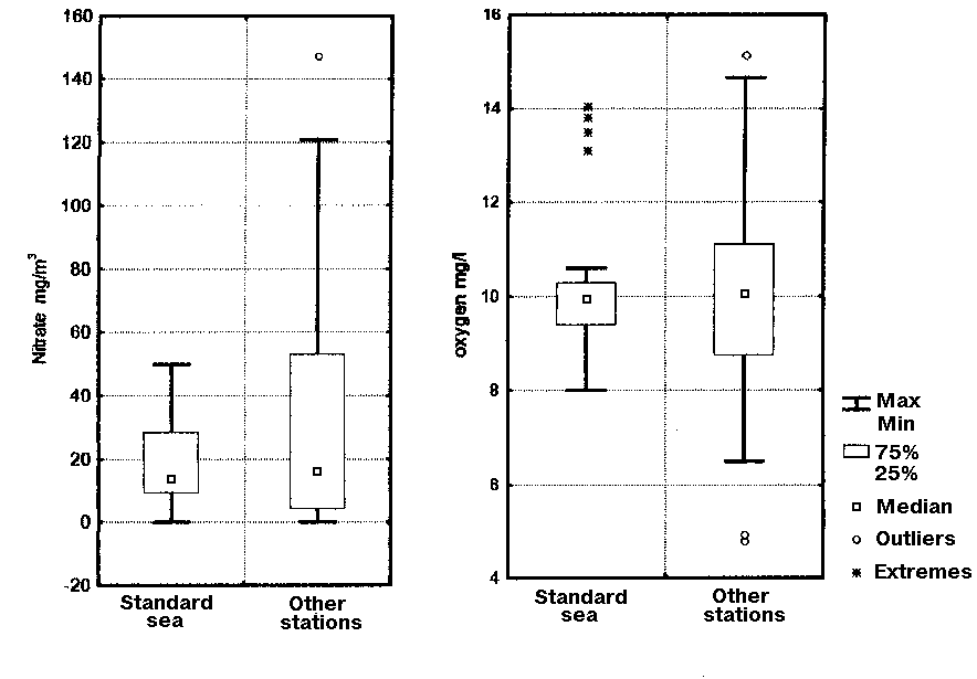
The similar situation was observed in our work [24] devoted to the analysis of the data obtained during ecological monitoring in Baltic Sea (Finnish Gulf) in 1979-83. At the analysis of likeness of phytoplankton specific structure the whole aggregate of samples has broken up to 2 groups. One of them contained samples taken on stations located, so to tell, on axes of Finnish Gulf, almost in equal distance from Estonian and Finnish shores. The second group was derived by samples selected in Narva Gulf or in adjacent area. Thus the likeness of specific structure of dominating species in the first group was higher on the average, i.e. phytoplankton community in these stations was a little more stable both in space and time. Moreover, in phytoplankton of Narva gulf there were microalgal species which are inherent for Narva river. This fact first of all explained difference between samples in second and first group. Therefore the first group was selected as standard group.

The analysis of hydrochemical data obtained in the same stations has shown that, as expected, on stations of the first group a pollutants content, controlled by the monitoring program, never reached those extreme values which were rather frequently observed in another stations. It is visible, for example on Fig.1, where the diagrams (box and whiskers plots) are given, showing limits of changes of nitrates and dissolved oxygen concentration in standard stations in comparison with the same changes in another stations

2.4. Microbiological indication of soil ecological state

The way of evaluation of soil ecosystems ecological state is based on the knowledge of adaptive properties of soil microbial system [11]. It was found that with according to degree of anthropogenic loading the communities of soil microorganisms can undergo four gradations: preservation of stability in community structure (zone of homeostasis), reallocation of dominating populations (zone of stress), priority development of stable populations (zone of resistance), complete suppression of growth and development of microorganisms in soil (zone of repression). The good experimental reproducibility of indicated adaptive zones allows to offer them as diagnostic indicators of degree of disturbing in soil coenoses as a result of abiotic factors action.

2.5. Evaluation of ecological state by indices of effectiveness of ecosystem functioning

The experience of searching for integrated indices of norm and pathology for ecosystems functioning [10, 18] suggests to select indices of their higher trophic levels as the function of response. The values of commercial fishes (bream, pike-perch, sturgeon and others) catch and productivity in Don river during last 50 years were applied for diagnostics of water ecosystem state [7]. The offered method of diagnostics assumed representation of the whole series of fishes catch and productivity observations not as absolute number, but as classes of values on scale “low-high number”. For this purpose all catch values was classified in 3-mark scale. Catch values included in interval from minimum value up to average between minimum and average-for-all-years values were estimated by a number 3; catch values in interval from average between maximum and average-for-all-years values up to maximum value were estimated by a number 1. Number 2 was assigned to intermediate catch values. After this boundary of norm and pathology on rating scale was entered: the catch (productivity)values, appreciated by numbers 2 and 3, are referred to low ones; and catch values with numbers 1 to high ones. Thus, ideas about relative norm of catch (productivity) state during some standard period of observations were used. The indicated norm was entered for use in a regional standardisation of chemical and thermal pollution, and also admissible water expenditures in water objects of Lower Don river (appropriate brief description and the references are resulted in section 3.2).

For human ecosystems, as the function of a response is possible, for example, quantitative indices of death rate can be offered, which in integrated aspect certainly reflect influence of environment on people health.

3. Ecological normalization and prediction on a basis of biotic of identifiers

3.1. ETL Method

The realisation of “biotic” approach to ecological standardisation requires a execution of the following research phases:

- creation of statistically representative bank of biological data concerning studying ecosystem;

- diagnostics of a ecosystem state on the scale “norm-pathology” by biotic identifiers for each observation;

-creation of bank of abiotic environmental data which potentially influence on biota ecological state and correspond to biological observations by time and place of sampling.

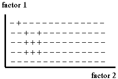
Fig. 2. Area of normal functioning (signs “plus”) in space of environmental factors

The collection of indicated ecological data can be visually represented as the following geometric image: in multidimensional space of biotic factors the collection of observations is represented as “cloud” of points, each of which is estimated by a marker of ecological state evaluation (in the simple case, there are two “marks” — “plus” (normal state) and “minus” (pathological state, Fig.2).

The aggregate of “good” points forms the area of normal functioning of ecosystem. It is the boundary of this area which represents research object in ETL method. To describe the method without unnecessary details, we shall accept additional suppositions simplifying a real picture: the area of normal functioning is one-way connected and adequately approximated by a multidimensional cube. Then projections of area of normal functioning on axes of abiotic factors space represent limits of a modification of each factor, an exit out of which transfers ecosystem from satisfactory to unsuccessful state. These limits are called ecologically tolerable levels (ETL) of factors and are determined by ETL method [19].

For real aggregates of observations boundaries of area of normal functioning are indistinct and blurred. Therefore in ETL method procedures of optimal image recognition, multidimensional statistical and determination [33] analysis are used.

If estimations of a state aren’t binary, then the method allows to receive the standards of various rigidity. The shift of boundary between estimations, which were declared as satisfactory and unsuccessful, changes boundaries of area of normal functioning in space of disturbing factors as well as ETL standards. Thus, there is a possibility to introduce the differentiated standards of admissible influences for various categories of natural objects (for example, preservation zones, recreational zones, economic territories, dumping zones, etc.).

Naturally, ETL standards obtained on the basis of estimations by various biotic identifiers can differ. For the choice of “true” standard it is necessary, as well as in case of selection of state estimations, either to select the priority identifier, or by applying a principle of the greatest rigidity [19] to select the most rigid standard.

ETL method allows:

— to select those acting factors from the whole set, which make the most significant contribution to ecological troubles of researched natural object;

— to rank the separate factors and their various sets by contribution to troubles degree;

— to calculate the ETL standards for the significant factors;

— to specify ecologically safe boundaries (ESB) for insignificant factors, inside which the ecosystem state in its previous history was certainly satisfactory;

— to calculate ETL standards for preceding, current, averaged, extreme, etc. values of abiotic factors;

— to build chronograms of seasonal and long-term ETL dynamics (for example, chronograms for ETL of water expenditures);

— to investigate a stability of harmful factors influence on ecosystem state;

— to discover an incompleteness of observations in current monitoring programs;

— to generate optimal paths of an ecosystem recovering from trouble states.

Concluding section, we shall once again underline a series of features distinguishing the ETL standards from the MAC standards:

— the selected boundaries are not universal, and reflect specificity of given region, its background characteristics and adaptive potential of concrete ecosystem biota;

— ETL of each factor is defined in view of influence of whole complete complex of abiotic factors on ecosystem, including all factors that have not be taken into account by monitoring programs;

— ETL standards are obtained not for isolated laboratory populations, but for all organisms really interacting in ecosystem;

— ETL take into account not only direct, but also indirect effects of influence;

— The ETL method allows to standardise non-substrate influence on ecosystems, for which MAC are not determined (more detailed description of ETL for temperature and acidification is told in the following section).

3.2. Examples of ETL calculation

In a series of works [7, 20, 21] results of ETL calculation for pollutants (chlororganic substances, pesticides, copper, zinc, nitrates, nitrites, ammonium, sediments, phenols, sulphates, chlorides) and for water expenditures are resulted. In the present section we shall illustrate the ETL method by example of standardisation of temperature and acidification in Don river, which can be used, for example, for analysis of global climate modification consequences or transglobal atmospheric transfers.

Table 2.

ETL values of water temperature and pH for ecosystems of Lower Don river (explanations are in the text).

The data about phytoplankton, zooplankton, periphyton, zoobenthos and catch and productivity of commercial fishes were used as biotic identifiers of an ecosystem state. By ETL method monthly and yearly averaged values of temperature and pH were standardised. Searching for the ETL standards of indicated factors was carried on in area both high and low values. In table 3 for each identifier ETL values for temperature and pH, which are significant for ecological troubles, i.e. satisfying to defined statistical criteria of ETL method, are resulted. As temperature is especially specific value for given observation site, the relative temperature is used in calculations, i.e. ratio of current temperature to yearly averaged temperature in given observation site. To receive ETL value of absolute temperature, it is necessary to multiply the value indicated in Table 2 by yearly averaged temperature in analysed observation site.

On Fig. 3 seasonal dynamics(changes) of a modification of relative temperature ESB and ETL in water objects of Lower Don on one of biotic identifiers is represented.

3.3. Ecological prediction

The prediction is carried out under the scenarios of potential disturbing influences. I.e., a prediction of ecological state of researched natural object is carried out by given values of abiotic factors. Offered method of prediction implies that some system of state estimations for researched ecosystem is given and that for the factors included in the scenario ETL values are known which are obtained by the same system of estimations and the same set of biotic identifiers. Then the compilation of the prediction becomes trivial, i.e. it is necessary to clarify, what side from boundary of normal functioning (or what side of ETL value) each of given in the scenario value of disturbing factors is found in. Thus, the state of the researched object is unsuccessful, if the value of only one factor from the scenario comes outside the ETL limits. On the other hand, the state is satisfactory, if values of all factors from the scenario are in the range of ETL. The example of application of offered prediction technique is contained in one of the authors’ works [8].

The work is supported by grants of Russian Fund of Basic Research N 95-04-11141à and N 97-05-64466.

Key words: ecosystem ecological state, biotic identifiers, abiotic factors, ecological standardisation.

References

1. Abakumov, V.A. Ecological modification and biocenosis development, In: Ecological Modification and Criteria for Ecological Standardisation, pp. 15-32, Gidrometeoizdat, St. Petersburg, 1992.

2. Abakumov, V.A. (ed.). Guide on hydrobiological monitoring freshwater ecosystems, Gidrometeoizdat, St. Petersburg, 1992.

3. Abakumov, V.A. & Sushenya, L.M. Hydrobiological monitoring of the state of freshwater ecosystem and ways to its improvement, In: Ecological Modification and Criteria for Ecological Standardisation, p. 33, Gidrometeoizdat, St. Petersburg, 1992.

4. Averintsev, V.G. An evaluation of seasonal dynamics of functional state in High-Arctic shallow ecosystem of the Frantz-Joseph Earth by ÀÂÑ- method, In: Problems of ecology in polar areas. Issue 2, pp. 23-24, Science, Moscow, 1991.

5. Bazzaz, F.A. Plant species diversity in old-field successional ecosystems in Southern Illinois, Ecology, 1975, 56, 485-488.

6. Beukema, J.J. An evaluation of the ABC-method as applied to macrozoobenthic living on tidal flats in the Dutch Wadden Sea, Mar. Biol.,1988, 99, 425-433.

7. Bulgakov, N.G., Dubinina, V.G., Levich, A.P. & Teriochin, A.T. Method of searching for correlation between hydrobiological indices and abiotic factors (using commercial fish), Biology Bulletin of the Russian Academy of Sciences, 1995, N 2, 218-225.

8. Bulgakov, N.G., Levich, A.P. & Maximov, V.N. The prediction of an ecosystem state in water objects of Lower Don, Biology Bulletin of the Russian Academy of Sciences, 1997 (in press).

9. Faschuk, D.Ya. Geographic-ecological model of sea reservoir. Autosummary of dissertation, Moscow, 1997

10. Fyodorov, V.D., Sakharov, V.B. & Levich, A.P. Quantitative approaches to problem of evaluation of norm and pathology of ecosystem, In: Man and Biosphere, pp.3-42, Moscow University Press, Moscow, 1981, Issue 6.

11. Guzev, V.S. & Levin, S.V. Perspectives of ecologico-microbiological expertise of soil state at anthropogenic influences, Pochvovedenie, 1991. N 9, 50-62.

12. Inagaki, H. & Lenoir, A. Une etude d’ecologie evolutive: application de la loi de Motomura aux fourmis, Bull. Ecol., 1974, 5, N 3, 207-219.

13. Israel, Yu.A. Ecology and control of natural environment state, Gidrometeoizdat, Moscow, 1984.

14. Lecordier, C. & Lavelle, P. Application du modele de Motomura aux peuplements de vers de terre: signification et limites, Rev. Ecol. Et Biol., 1982, Sol., 19, N 2, 177-191.

15. Levich, A.P. A structure of ecological communities, Moscow University Press, Moscow, 1980.

16. Levich, A.P. A Biological Concept of Environmental Control, Doclady Biological Sciences, 1994, 337, N 2, 360-362.

17. Levich, A.P. Phenomenology, application and origin of rank distributions in biocoenoses and ecology as a source of ideas for technocoenoses and economics, In: Mathematical description of coenoses and regularity of technetics, pp.93-105, Centre of system researches, Abakan, 1996.

18. Levich, A.P. & Fyodorov, V.D. Explication of norm concept and whole properties of ecosystems, In: Man and Biosphere, pp.3-16, Moscow University Press, Moscow, 1978, Issue 2.

19. Levich, A.P. & Teriochin, A.T. Method of calculation of ecologically tolerable levels of influences on ecosystems (ETL method), Vodnye resursy, 1997, N 3, 328-335.

20. Levich, A.P., Teriochin, A.T., Bulgakov, N.G., Abakumov, V.A., Eliseev D.A., Maximov, V.N. & Katchan L.K. Ecological control of water objects in Lower Don by biotic identifiers of plankton, periphyton and zoobenthos, Moscow State University Bulletin. Biological series, 1996. N 3, 18-25.

21. Levich, A.P., Bulgakov, N.G., Abakumov, V.A. & Teriochin A.T. Determination of ecologically tolerable levels of water expenditures by hydrobiological indices, Moscow State University Bulletin. Biological series, 1997 (in press).

22. Maximov, V.N. Problems of complex evaluation of natural water quality (ecological aspects), Hydrobiological Journal, 1991, 27, N 3, 8-13.

23. Maximov, V.N. Rank method of evaluation of communities likeness at the analysis of ecosystem state, In: Ecological Modification and Criteria for ecological standardisation, pp. 329-333, Gidrometeoizdat, St. Petersburg, 1991.

24. Maximov, V.N, Andryuschenko, V.V. , Morozov, V.I. & Simonov, A.I. Evaluation of sea ecosystem state by the data of chemical and biological monitoring, In: Problems of background monitoring of natural environment state, pp.140-146, Gidrometeoizdat, St. Petersburg, 1987, Issue 5.

25. Maximov, V.N., Dzhabrueva, L.V., Bulgakov, N.G. & Teriochin, A.T. Concept of detection of stress states in water ecosystems by method of rank distributions and ecologically tolerable levels of pollutants for reservoirs of Elista river, Water resources, 1997, 79-85.

26. Maximov, V.N., Bulgakov, N.G. & Dzhabrueva, L.V. Rank distributions of microalgal size-morphological groups in periphyton and their connection with level of reservoir pollution, Biology Bulletin of the Russian Academy of Sciences,1997 (in press).

27. McManus, J.W. & Paulv, D. Measuring ecological stress: variations on theme by R.M. Warwick, Mar. Biol., 1990, 108, N 2, 210-221.

28. Meire, P.M. & Deren, J. Use of the abundance-biomass comparison method for detecting environmental stress: some considerations based on intertidal macrozoobenthos and bird communities, J. Appl. Ecol., 1990, 27, N 1, 210-221.

29. Nosov, V.N., Bulgakov, N.G. & Maximov, V.N. Building the function of desirability in the course of analysis of the ecological monitoring data, Izv. Acad. Nauk Biol., 1997,N 1, 69-74.

30. Organisation and realisation of regime observations for pollution of surface dryland waters on Russian Hydrometeorological Committee web. Methodical instructions. Nature protection. Hydrosphere. Managing document RD, Gidrometeoizdat, St. Petersburg, 1992.

31. Sakharov, V.B. & Ilyash, L.V. Application of method of desirability function to analysis of results of studying of zinc and chromium influence on phytoplankton of Rybinskoe reservoir, Biological sciences, 1982, N 8, 65-68.

32. Sirotkina, N.V. & Levich, A.P. Influence of heavy metals on specific and overspecific structure of phytoplankton community of Rybinskoe reservoir, In: Man and Biosphere, pp.17-41, Moscow University Press, Moscow, 1979.

33. Tchesnokov, S.V. Determination analysis of social and economic data, Nauka, Moscow, 1982.

34. Vorobeytchik, E.L., Sadykhov, O.F. & Farafontov, M.G. An ecological standardisation of technogenic pollution of terrestrial ecosystems, Nauka, Ekaterinburg, 1994.

35. Warwick, R.M. A new method for detecting pollution effects on marine macrobenthic communities, Mar. Biol., 1987, 95, N 2, 193-200.