QUANTUM-MECHANICAL UNCERTAINTY RELATIONS AS A CONSEQUENCE OF THE POSTULATES OF N.A.KOZYREV’S CAUSAL MECHANICS; FORCES IN CAUSAL MECHANICS
L. S. Shikhobalov
This paper consists of four independent sections. In the first one Heisenberg’s uncertainty relations are derived on the basis of the fundamental postulates of N.A.Kozyrev’s causal mechanics. The second section contains a definition of the course of time c2 differing from that introduced by N.A.Kozyrev. In the third section possible generalizations of Kozyrev’s expressions for the additional forces acting in causal links in causal mechanics are proposed. The fourth section analyses the inaccuracy of force representation in classical mechanics related to the neglect of time intervals between causes and effects.
1. Causal mechanics and the quantum-mechanical uncertainty relations
N.A.Kozyrev’s causal mechanics (Kozyrev 1991) begins with the postulates claiming that in an elementary cause-effect link the cause and effect points are separated by an arbitrarily small but nonzero space and time differences dx and dt whose ratio is a fundamental constant called the course of time c2:
![]() . (1.1)
. (1.1)
The constant c2 is assumed to be pseudoscalar. Its pseudoscalarity is related to the same property of the quantity dt. However, the statement that dt is pseudoscalar, is, in our view, not sufficiently justified. To “avade” the question of whether dt is a pseudoscalar or a true scalar, let us pass in law (1.1) to the magnitudes of the quantities:
![]() . (1.2)
. (1.2)
The physical meaning of the quantities dx and dt is not described in detail in causal mechanics. We assign them the meaning allowing one to establish a relation between causal mechanics and quantum physics.
Let space and time form a unified four-dimensional manifold possessing the proper Euclidean geometry including both space and time variables (in what follows it does not matter which global geometry, proper Euclidean or pseudoeuclidean, is used, since the spatial and temporal quantities are considered separately in the present section).
We define a “collision” as an interaction of material points (particles) that they approach each other to the minimum possible spatial and temporal distances. It should be noted that the minimum distances between particles may be different in different “collision” acts, but they are undoubtedly nonzero since in a Euclidean continuum different points are always separated by a nonzero interval.
Assume that the space and time coordinates of “colliding” material points are independent random variables and that the quantities к dxЅ and к dtЅ are quantum-mechanical uncertainties (i.e., root-mean-square values) in space and time distances between the “collided” particles:
![]() , (1.3)
, (1.3)
where ![]() , t1,
, t1, ![]() , t2 are the spatial radius-vectors and time coordinates of the “collided” particles; the bars denote the procedure of averaging over all the possible values.
, t2 are the spatial radius-vectors and time coordinates of the “collided” particles; the bars denote the procedure of averaging over all the possible values.
Assume that the random quantities ![]() and
and ![]() , as well as
, as well as ![]() and
and ![]() , are characterized by the same distribution densities and average values. The space-time point coinciding with the average position of both particles, will be called the collision point. It is this point that in a macroscopic description is considered to be the place where the two particles “collide”. The spatial radius-vector
, are characterized by the same distribution densities and average values. The space-time point coinciding with the average position of both particles, will be called the collision point. It is this point that in a macroscopic description is considered to be the place where the two particles “collide”. The spatial radius-vector ![]() and the time coordinate t of the collision point are
and the time coordinate t of the collision point are
![]() . (1.4)
. (1.4)
The root-mean-square deviations from the collision point are equal for the two particles due to identity of their density distributions, and they, in both space and time directions, are, respectively,
 (1.5)
(1.5)
By (1.3) - (1.5) and due to independence of the random quantities ![]() and
and ![]() one can write:
one can write:
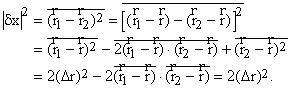
Hence the particle spatial position uncertainty is connected with the quantity п d xп by the relation
![]() (1.6)
(1.6)
Similarly for the particle’s temporal coordinate uncertainty one can obtain the following relation involving п d tп :
![]() (1.7)
(1.7)
While describing a “collision” at the macroscopic level, a single point introduced above by (1.4) is assumed to be the force application point for both particles. Meanwhile, the real positions of particles in space and time and consequently their force application points may not coincide with the collision point. The inaccuracy of the force application points determination leads to the inaccuracies of particle energies and momenta. Besides, the energy determination error is equal to the work to be done by the force displacing a particle from the collision point to that of its real location. And the momentum determination error is equal to an additional momentum which the particle should have gained under the action of the above force for a time interval between the real interaction instant and that corresponding to the collision point. Thus, the inaccuracies of energy and momentum determination in a separate “collision” act are equal to ![]() and
and ![]() , respectively, for one particle, and
, respectively, for one particle, and ![]() and
and ![]() for the other, where
for the other, where ![]() and
and ![]() are forces acting on the first and second particles. The root-mean-square values of these quantities may be identified with quantum-mechanical uncertainties in particle energies and momenta. Let us calculate them.
are forces acting on the first and second particles. The root-mean-square values of these quantities may be identified with quantum-mechanical uncertainties in particle energies and momenta. Let us calculate them.
Assume that the particles interact by the forces described by Newton’s classical mechanics, i.e. the forces which are equal in magnitude, oppositely directed and have a common line of action, namely, the straight line passing through both particles (the forces introduced in causal mechanics are neglected due to their smallness). Such forces may be represented in the form
![]() (1.8)
(1.8)
where F is the magnitude of the forces ![]() and
and ![]() and
and ![]() is the direction unit vector; the plus and minus signs correspond to the cases of particle repulsion and attraction, respectively.
is the direction unit vector; the plus and minus signs correspond to the cases of particle repulsion and attraction, respectively.
While calculating the energy uncertainties, we restrict ourselves to the case when the particles in “collision” are situated on the same line with the collision point (whose position may be different for different “collisions”). Since in this case the forces ![]() and
and ![]() are oriented along the same line, the direction unit vector in (1.8) coincides up to a sign with the vectors
are oriented along the same line, the direction unit vector in (1.8) coincides up to a sign with the vectors ![]() and
and ![]() , hence (1.8) may be rewritten in the form
, hence (1.8) may be rewritten in the form
![]() (1.9)
(1.9)
(here and in Eq. (1.11) presented below the sign of ![]() may differ from that in formula (1.8)). For such a representation of the forces
may differ from that in formula (1.8)). For such a representation of the forces ![]() and
and ![]() one easily calculates the energy value uncertainty D E, the same for both particles:
one easily calculates the energy value uncertainty D E, the same for both particles:
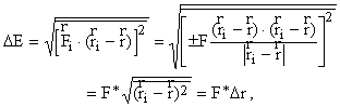 (1.10)
where F* is the value of F at a certain mean point; i = 1, 2; here the mean-value theorem and the first formula from (1.5) are used.
Now let us calculate the momentum uncertainty. Aiming to compare the result to be obtained with the corresponding result of quantum mechanics, we perform calculations in the one-dimensional case, as was done in the book by Landau and Lifshitz (1989). Let the “colliding” particles and the collision point be situated on a single line parallel to the z coordinate axis. Then the forces ![]() and
and ![]() described by (1.8) can be represented in the form
described by (1.8) can be represented in the form
![]() , (1.11)
, (1.11)
where ![]() is the direction unit vector of the z axis. In this case the uncertainty D pz of the momentum z component, having the same value for both “colliding” particles, is
is the direction unit vector of the z axis. In this case the uncertainty D pz of the momentum z component, having the same value for both “colliding” particles, is
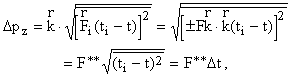 (1.12)
where F** is the value of F at a certain mean point; i = 1, 2; the mean-value theorem and the second formula from (1.5) are used. In this case the z coordinate uncertainty D z, having the same value for both colliding particles, is
![]() , (1.13)
, (1.13)
where z1, z2, z are the z coordinates of the particles in “collision” and that of the collision point, respectively.
Let us specify the values of the forces ![]() and
and ![]() . We shall assume that the particles bear electric charges e or -e (-e being the electron charge), interact only by electric forces and, while “colliding”, are mutually at rest. In this case their interaction is performed by the Coulomb forces described by the expression (1.8), with the magnitude
. We shall assume that the particles bear electric charges e or -e (-e being the electron charge), interact only by electric forces and, while “colliding”, are mutually at rest. In this case their interaction is performed by the Coulomb forces described by the expression (1.8), with the magnitude
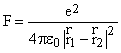 ,
,
where ![]() is the vacuum permittivity. In what follows we use only that magnitude value of forces which corresponds to the particle spacing
is the vacuum permittivity. In what follows we use only that magnitude value of forces which corresponds to the particle spacing ![]() equal toп d xп . It is this force magnitude value that is further designated as F:
equal toп d xп . It is this force magnitude value that is further designated as F:
 . (1.14)
Now let us form the product of the force magnitude F and the uncertainties in the space and time coordinates of the particles. Taking into account the dependences (1.6), (1.7), (1.14) and the definition of the course of time ![]() , we obtain
, we obtain
![]() (1.15)
(1.15)
where ![]() is the fine structure constant;
is the fine structure constant; ![]() is the Planck constant and c is the velocity of light in vacuum.
is the Planck constant and c is the velocity of light in vacuum.
It is evident that the parameters F* and F** involved in Eqs. (1.10) and (1.12), can be set equal to F. Hence from (1.10), (1.12), (1.13), (1.15) it follows that
![]() (1.16)
(1.16)
One of the uncertainty relations of quantum mechanics, written for the minimum possible values of the uncertainties, is of the form
![]() (1.17)
(1.17)
Comparing the second relation of (1.16) with (1.17), we find:
![]() km/s. (1.18)
km/s. (1.18)
The fact that the constant c2, the fundamental quantitative characteristic of causal mechanics, is represented in the form of a product of fundamental constants, confirms the validity of one of the starting points of Kozyrev’s theory, namely, that this constant is fundamental.
The above numerical value of the constant c2 is in agreement with the value obtained by N.A.Kozyrev experimentally by measuring additional forces in mechanical systems (Kozyrev 1991, pp. 367, 382). The fact that the experimental value of c proved to be precisely the one, allowed him to adopt the relationship п c2п = a c as an empirical fact.
The result expressed by (1.18) allows some points of quantum mechanics to be reviewed. The origin of the fine structure (dimensionless, fundamental) constant has been troubling physicists for long. Thus, R.Feynman (1985) named the question of how this number appears, one of the greatest damned mysteries of physics: a magic number which is given to us and which man does not understand at all. Relations (1.18) lift the veil of mystery around this number. According to N.A.Kozyrev, “...the presence of the dimensionless constant ![]() ceases to be mysterious and becomes natural as a ratio of two fundamental velocities” (Kozyrev 1991, p. 367).
ceases to be mysterious and becomes natural as a ratio of two fundamental velocities” (Kozyrev 1991, p. 367).
Equations (1.18) enable one to refine and reinterpret the uncertainty relation for energy and time. This relation, as applied to the minimum possible values of the uncertainties, is conventionally written in the form
![]() (1.19)
(1.19)
This relation, unlike (1.17), does not set an exact lower bound of the product of uncertainties but only its order of magnitude. The very quantities entering into (1.19) are treated differently from those appearing in (1.17). This is related to the fact that in quantum mechanics time is considered to be a determinate but not random variable. Hence the quantities D E and D t are not understood conventionally, i.e., they are not regarded as root-mean-square deviations but, instead, as an energy measurement error and a duration of its measuring respectively (De Broglie 1982, Demutsky and Polovin 1992). It is easy to see that the difference in interpretations of quantum mechanical dependences (1.17) and (1.19) contradicts the relativistic symmetry of space and time. Equations (1.18) allow this contradiction to be eliminated. They and the first equality from (1.16) lead to the uncertainty relation for energy and time in the “standard” form relating to one another the minimum possible values of the root-mean-square deviations of the corresponding variables:
![]() (1.20)
(1.20)
Equations (1.18) and (1.15) yield one more uncertainty relation:
![]() , (1.21)
, (1.21)
where a value with the dimension of action stands at the left-hand side.
Restrictions on the possible values of the quantities ![]() and
and ![]() can be obtained provided that the energy uncertainty does not exceed the rest energy of an electron:
can be obtained provided that the energy uncertainty does not exceed the rest energy of an electron:
![]() (1.22)
(1.22)
where me is the electron mass. This condition and Eqs.(1.6), (1.7), (1.14), (1.20), (1.21) lead to the following inequalities:
 (1.23)
where the quantity on the right side of the first inequality is equal to half the so-called classical radius of an electron.
The present section departs from the division of interacting material points into a cause and an effect, being of importance in causal mechanics (as the effect always comes after the cause). The interacting particles are equivalent in the above considerations and cannot be consistently divided into a cause and an effect, e.g., their time coordinates in “collision” equally probably satisfy both inequalities t1 > t2 and t2 > t1.
Making use of the uncertainty relation (1.17), we have proved the validity of Kozyrev’s law (1.2) and confirmed that the course of time c2 has just the value which N.A.Kozyrev ascribed to it on the basis of the results of macroscopic experiments. If the law (1.2), involving the constant c2 given by (1.18), were assumed to be a fundamental postulate, the uncertainty relations (1.17), (1.20), (1.21) might be easily obtained. This means, in particular, that the quantum-mechanical uncertainty relations may be regarded as a consequence of the postulates of causal mechanics.
From the content of the present section it can be concluded that Kozyrev’s causal mechanics is in agreement with quantum physics. Moreover, causal mechanics results in a new interpretation of Heisenberg’s uncertainty relations. The latter may be treated as a consequence of the uncertainty in the space-time intervals in particle “collisions”. The uncertainties obey the law (1.2) with the constant c2 equal in magnitude to ![]() . This interpretation may obviously make us revise our attitude to the other conceptual statements of quantum mechanics as well.
. This interpretation may obviously make us revise our attitude to the other conceptual statements of quantum mechanics as well.
2. On the time characteristic c2 in N.A.Kozyrev's theory
An experiment for measuring the course of time c2 was carried out by N.A.Kozyrev by weighing a rotating gyroscope with a vertically oriented axis (Kozyrev 1991). When vertical vibrations were introduced into the balance-gyroscope system, a change of the gyroscope weight was observed by the value of D F proportional to its weight F and the linear rotation speed v of the rotor; the value of the parameter c2 was calculated by the formula
![]() (2.1)
(2.1)
and turned out to be about 2200km/s (Kozyrev 1991, pp.366-367, 382). N.A.Kozyrev treated this fact as appearance of additional forces neglected in classical mechanics. He postulated c2 to be a pseudoscalar, since the effect changed sign when the physical system under investigation was replaced by a mirror-symmetric one.
The course of time c2 is defined in causal mechanics as the rate of causal action realized in an elementary cause-and-effect link comprising two material points, those of the cause and the effect:
![]() , (2.2)
, (2.2)
where d x and d t are arbitrarily small but nonzero space and time differences between the cause and effect points.
This definition assigns a clear physical meaning to the most important characteristic of time in causal mechanics. The validity of just this definition is supported by the results of the previous section where the quantity c2 was proved to be a fundamental constant. Nevertheless, the above definition has a number of shortcomings.
1. The course of time c2 is determined by Eq. (2.2) in terms of the quantities d x and d t eluding a direct experimental measurement.
2. Equation (2.2) is inconsistent with a pseudoscalar nature of c2 (N.A.Kozyrev’s assumption that the time interval d t is a pseudoscalar, is not sufficiently justified in his papers (Kozyrev 1991) and therefore cannot be taken for granted).
3. The definition under consideration leads to an inconsistency between the instantaneous character of action transmission via time through cosmic distances (Kozyrev and Nasonov 1978, 1980) and the finiteness of the action transmission velocity in an elementary cause-and-effect link.
4. Kozyrev (1991) has not presented a strictly logical transition from the definition (2.2) to the additional force formula (2.1) (such a transition is most likely impossible in principle, since with only a single scalar quantity (c2) available no unambiguous conclusion concerning a vector quantity, i.e., the additional force, can be made). Hence the quantity c2 appearing in (2.1) must not necessarily coincide with that defined by (2.2).
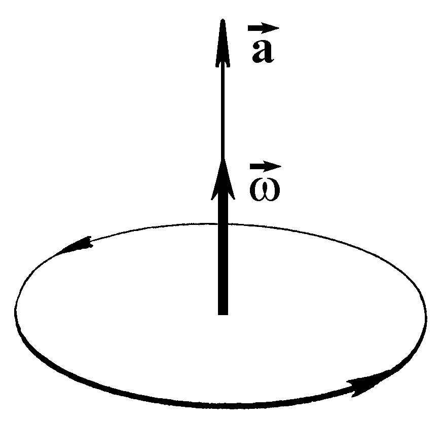
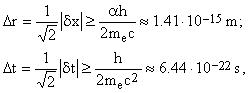
Fig.1. A pair of collinear vector ![]() and pseudovector
and pseudovector ![]() : The shown direction of the pseudovector
: The shown direction of the pseudovector ![]() corresponds to the marked circle round travel direction in a right coordinate system.
corresponds to the marked circle round travel direction in a right coordinate system.
In connection with the shortcomings of this definition it would be reasonable to try to formulate another definition of the course of time, retaining the essential features of the quantity c2 described by Kozyrev (1991) but free of these shortcomings. Such a definition is suggested below.
Based on the propositions of causal mechanics, we shall assume that time interacts in different ways with right- and left-handed physical systems by its active properties. A pair (![]() ) consisting of a vector
) consisting of a vector ![]() and a pseudovector
and a pseudovector ![]() collinear to each other, is one of the simplest mathematical objects distinguishing the right from the left (Fig.1). (A simple example: a motion in the direction pointed by the vector
collinear to each other, is one of the simplest mathematical objects distinguishing the right from the left (Fig.1). (A simple example: a motion in the direction pointed by the vector ![]() combined with a rotation defined by the pseudovector is right-hand-screw if the directions of
combined with a rotation defined by the pseudovector is right-hand-screw if the directions of ![]() and
and ![]() coincide and left-hand-screw otherwise.) Assume that the course of time is described exactly by such a mathematical object. Then it may obviously manifest itself in physical systems whose kinematics is characterized by a similar vector pair. This is just the case in the experiment with a vibrating gyroscope described above, where such a kinematic pair is formed by the gyroscope acceleration
coincide and left-hand-screw otherwise.) Assume that the course of time is described exactly by such a mathematical object. Then it may obviously manifest itself in physical systems whose kinematics is characterized by a similar vector pair. This is just the case in the experiment with a vibrating gyroscope described above, where such a kinematic pair is formed by the gyroscope acceleration ![]() due to its vibration and the angular velocity of its rotation
due to its vibration and the angular velocity of its rotation ![]() (here a is a scalar,
(here a is a scalar, ![]() is a pseudoscalar,
is a pseudoscalar, ![]() is the direction unit vector of the rotation axis).
is the direction unit vector of the rotation axis).
It can be assumed that the action of the physical properties of time on the gyroscope results in appearance of the addition D a and D w to the values of a and w , which are monotonic functions of these values, satisfy the condition D a = D w = 0 if aw = 0 and have signs depending on the mutual orientation of the vectors ![]() and
and ![]() . Then we can write down in the linear approximation in a and
. Then we can write down in the linear approximation in a and ![]() :
:
![]() , (2.3)
, (2.3)
where ka and kw are dimensional coefficients; the signs are positive for one mutual orientation of the vectors ![]() and
and ![]() and negative for the other.
and negative for the other.
In gyroscope vibration its acceleration ![]() regularly changes its sign, whereas the angular velocity
regularly changes its sign, whereas the angular velocity ![]() remains unchanged. The time average of the addition D a turns out to be nonzero despite the fact that the average acceleration being zero. This is related to the fact that the sign of D a is the same for any half-period of vibration because it depends on both the sign of a and the mutual orientation of
remains unchanged. The time average of the addition D a turns out to be nonzero despite the fact that the average acceleration being zero. This is related to the fact that the sign of D a is the same for any half-period of vibration because it depends on both the sign of a and the mutual orientation of ![]() and
and ![]() changing together with the sign changing of a. Multiplying the mean value of D a by the gyroscope rotor mass, we obtain the mean value of the additional force acting on the gyroscope:
changing together with the sign changing of a. Multiplying the mean value of D a by the gyroscope rotor mass, we obtain the mean value of the additional force acting on the gyroscope:
![]() . (2.4)
. (2.4)
Here the relation w = v/ R is used; besides, the rotor mass is taken to be equal to the whole gyroscope mass F / g as it was done by Kozyrev (1991); R and v are the mean values of the rotor radius and its linear rotation velocity, respectively; F is the gyroscope weight; g is the free fall acceleration; an overbar denotes the time averaging operation. We do not specify the sign of D F , since the observable may always be fited by choosing the required sign in (2.3). The quantity D F may be obviously interpreted as a change of the gyroscope weight.
Let us compare (2.4) with the relation (2.1) obtained experimentally. It is seen that Eq.(2.4) incorporates the same dependence of the additional force on the linear rotation velocity of the rotor v and the gyroscope weight F as does the relation (2.1). This suggests that the first equality from (2.3) should be valid, since it is just the basis for Eq.(2.4). It should be emphasized that a distinction between the factors by vF in Eqs. (2.1) and (2.4) does not argue against this conclusion. The point is that the relation (2.1), being just an expression of particular experimental data, is of restricted nature. In particular, it neglects a dependence of the additional force on vibration intensity and on the geometric parameters of the gyroscope, which should occur in reality and is apparently taken into account by just the above factor in Eq.(2.4).
Thus, we have confirmed the validity of the first equality from (2.3). It is clear that the coefficient ka appearing in this equality may depend on the vibration characteristics and the gyroscope size. Assume that the second equality in (2.3) holds as well and the coefficient kw in it depends on the system properties in the same way as the coefficient ka (D w was not measured by Kozyrev, hence this assumption cannot be compared with the experimental data). Then the ratio D a/ D w is a pseudoscalar having the dimension of velocity and independent of the specific properties of the system under study.
It is natural to adopt the quantity D a/ D w to be the course of time ![]() . One easily assures that it is free of the mentioned shortcomings of the “old” definition based on the relation (2.2).
. One easily assures that it is free of the mentioned shortcomings of the “old” definition based on the relation (2.2).
The proposed approach to defining the course of time admits extension to physical systems unrelated to rotating bodies. Other quantities, e.g., energy flux density and the density of volume force moments, can play for such systems the same role as the pair (![]() ).
).
Remark. The content of the present section follows a manuscript of April 1979. The manuscript was discussed with N.A.Kozyrev who made the following two remarks.
1. In the case depicted in Fig.1 the momentum conservation law appears to be violated due to an uncompensated force acting on the system if ![]() is an acceleration. Meanwhile, the validity of this law has been verified to a high accuracy in special experiments when both the source of vibration and the gyroscope were placed on the same balance pan. In such experiments additional forces were not detected.
is an acceleration. Meanwhile, the validity of this law has been verified to a high accuracy in special experiments when both the source of vibration and the gyroscope were placed on the same balance pan. In such experiments additional forces were not detected.
Fig.2. A possible system of vectors for two interacting objects.
2. Equation (2.4) contains the rotor radius R. To bring it to the form (2.1), it is necessary to assume that ka ~ R. However, in such a case the physical meaning of formula (2.3) is unclear. Experiments with gyroscopes whose rotor had the shape of a thin-walled glass (so that the condition R є const was fulfilled to a good accuracy), as well as an analysis of planet figure asymmetries and an investigation of the latitudinal dependence of the gyroscope weight change effect convince that the ratio v/R є w in formula (2.4) should be replaced by the linear velocity v of the points of the rotor.
Figure 2, depicting a possible system of vectors for the cause-and-effect link as a whole, answers N.A.Kozyrev's first remark. It is seen that the uncompensated forces are absent in such a system and the momentum conservation law remains valid. However, the author has no answer to the second remark.